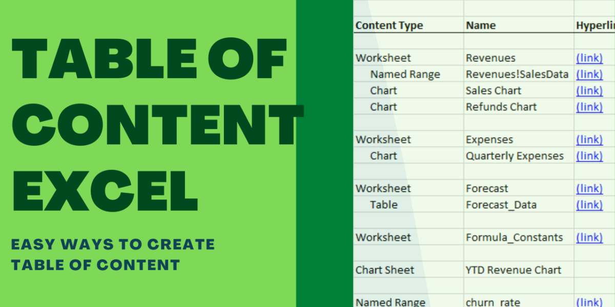
Want to organize all the worksheets in your Excel workbook? Try creating a table of contents. It makes it easy to find specific sheets, especially if your Excel file contains hundreds of them. Unfortunately, Excel doesn’t have a one-click feature for creating a table of contents, but there is a way!
Why You Should Add a Table of Contents to Excel
What would you do if you had hundreds of sheets in an Excel workbook and needed to find a specific one for updating or modifying data? Searching manually would take too much time. But, if you create a table of contents, you can easily navigate through the workbook and quickly find the sheet you need.
As an SEO content writer, I sometimes work with and manage large Excel files containing keyword data. With a table of contents, I can easily jump to the exact Excel sheet where the required information is stored, saving a lot of time and effort. It also eliminates the need to scroll through countless sheets and tabs.
A table of contents helps you maintain a structured layout by organizing related worksheets and sections logically, improving the overall user experience. It also makes it easier for your team members to find specific sections for input and review. Additionally, you can minimize errors by reducing the chances of accidentally modifying unrelated data.
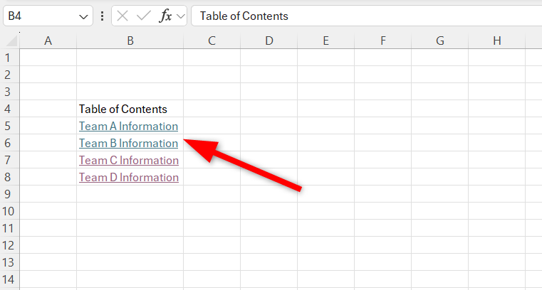
I’ll be using Microsoft Excel 365 for this demonstration. My workbook already contains four worksheets: Team A, Team B, Team C, and Team D.
Manually Add Table of Contents to Excel
To create a table of contents manually, first decide where you want to place it. It’s recommended to create a new worksheet for the table of contents to make it easier to locate and manage.
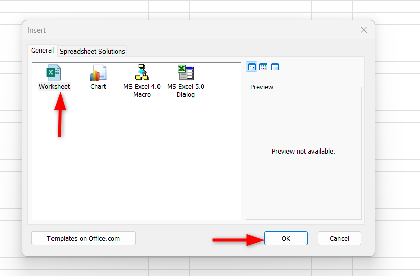
To create a new sheet, right-click on any existing worksheet name and click on “Insert,” then select “Worksheet.” Alternatively, you can press Shift+Alt+F1.
Next, select the cell where you intend to add the hyperlink, such as B5 (or any cell you prefer).
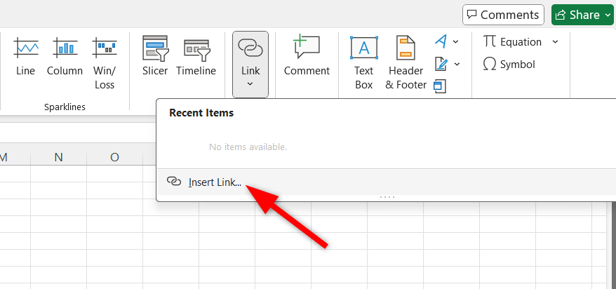
After selecting the cell, go to the Insert tab, click on the “Link” drop-down item, and select the “Insert Link” option to display the Insert Hyperlink dialog box. You can also access it using the Ctrl+K shortcut.
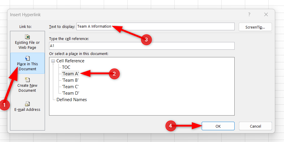
Navigate to the Place In This Document section, select your preferred sheet, and then type the text you want to display for the hyperlink. After doing this, press “OK” to insert the link.
Repeat the process for the other sheets.
That’s it! Now you have clickable links that will take you directly to the corresponding sheets when clicked.
Use Hyperlink Function/Formula
Another way to manually add a table of contents in Excel is by using the Hyperlink Function. In this method, you need to type all the names of your sheets and add hyperlink formulas to each one individually.
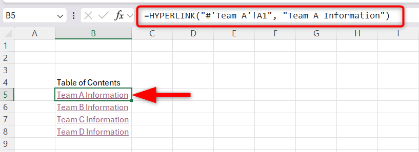
To get started, choose the cell where you want the TOC to appear and enter the following formula:
=HYPERLINK("#'WorkSheetName'!A1", "FriendlyName")
Here, “WorkSheetName” is the name of the worksheet for which you want to create a link. The “#” symbol identifies the worksheet, and the exclamation mark “!A1” represents the cell location on the targeted worksheet. Lastly, “FriendlyName” variable represents the name that will be displayed in the table of contents.
Repeat this process for the other sheets using the same formula.
Automatically Build Table of Content
You can automatically create a table of contents using Excel’s Power Query tool. With this tool, you can list hundreds of sheets on a specific sheet with just a few clicks and create hyperlinks that will take you directly to each respective sheet when clicked.
For a smooth connection in Power Query, I’d recommend that you pause your OneDrive sync with the workbook. You should also ensure that your workbook is saved and temporarily disable sharing.
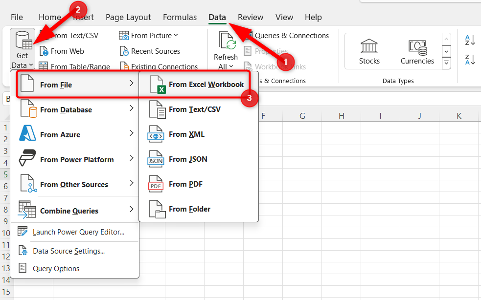
To get started, go to the Data tab in Excel. Click on “Get Data,” then select “From File” and hit the “From Excel Workbook” option.
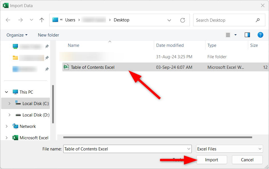
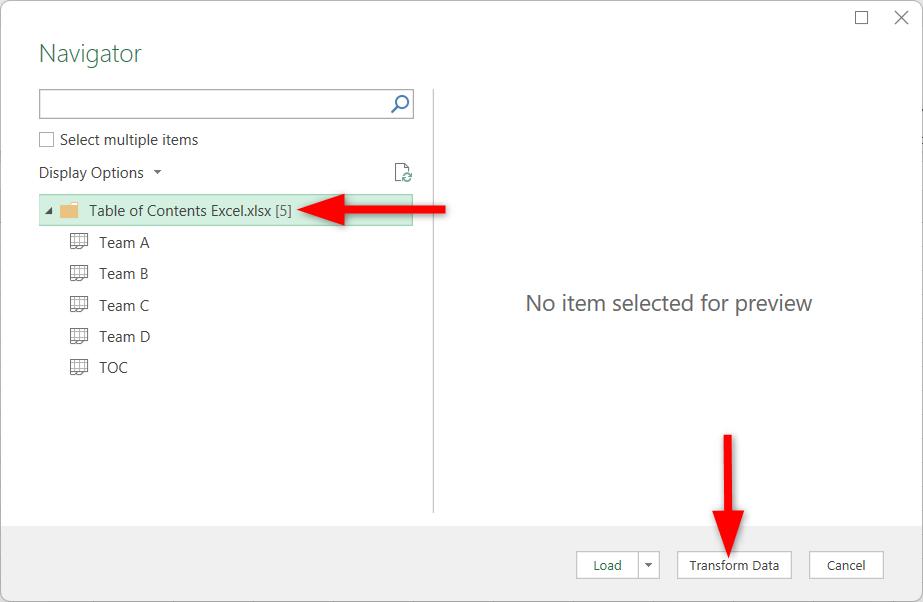
A dialog box will appear where you can select the workbook you’re currently working in. Once you’ve selected it, click “Import.”
Instead of choosing a specific table or sheet from the list that appears, select the name of the workbook itself. Then, click on “Transform Data.”
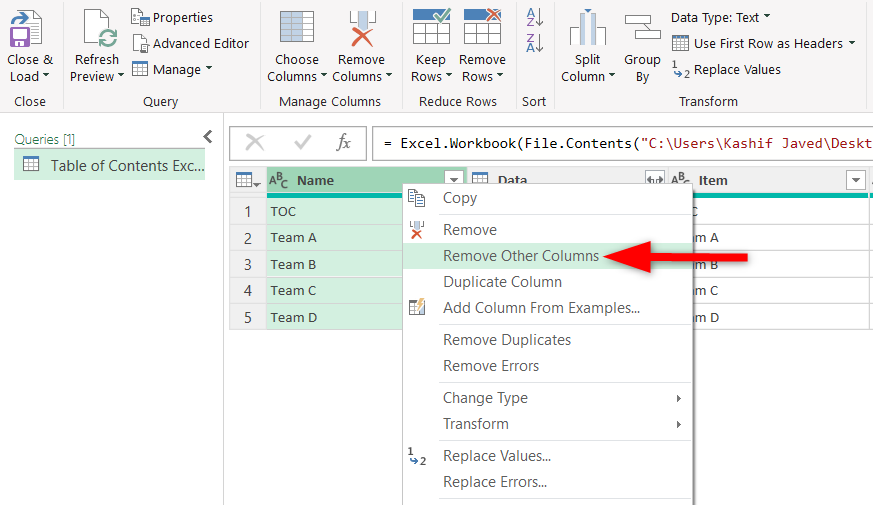
You will now see a list of all the sheets, tables, and defined names within the workbook. Since we only want the sheet names, apply a filter to show only the sheets from the “Kind” option.
Next, right-click on the “Name” column (which contains the sheet names) and select “Remove Other Columns.” This step leaves you with just one column that lists all the names of the sheet.
You can also rename your header to any preferred name. After making these changes, click on the “Close & Load To” option.
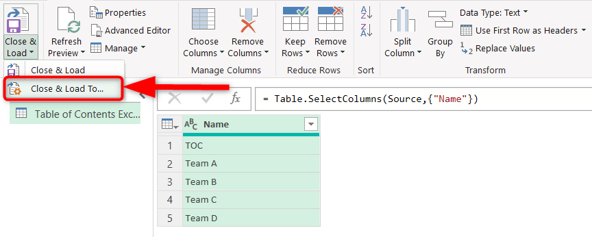
Select “Existing Worksheet” and enter the cell where you want the list to start (e.g., cell A1 or B5).
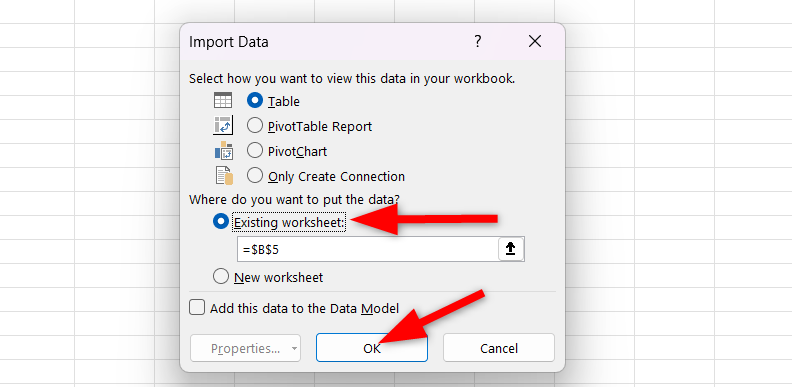
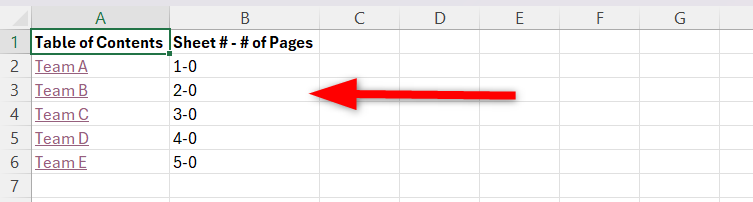
You’ll now have a collection of all the sheet names in your workbook.
The last step is to create hyperlinks for the sheet names using the hyperlink formula. When you create a hyperlink for the first sheet and press Enter, all the sheet columns will automatically update with their hyperlinks. If not, you can simply drag the fill handle to apply the formula to all rows in your table of contents.
You can create hyperlink using the following formula:
=HYPERLINK("#'"&[@WorkSheetName]&"'!A1", [@FriendlyName])
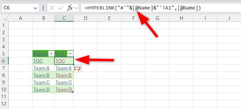
Now, if you click on any of the hyperlinks, it will take you straight to the corresponding sheet in your workbook.
Auto Refresh Sheet
One of the great benefits of using Power Query is that you can easily update your table of contents whenever you add or remove sheets from your workbook.
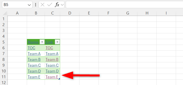
For example, I’ve added a new sheet to my workbook and saved it with the name “Team E.” Now I want this sheet to appear in the table of contents with its hyperlink.
To update the outline, simply go back to the master sheet and double-click on the “Table of Contents” Excel query that is displayed to the right of your workbook.
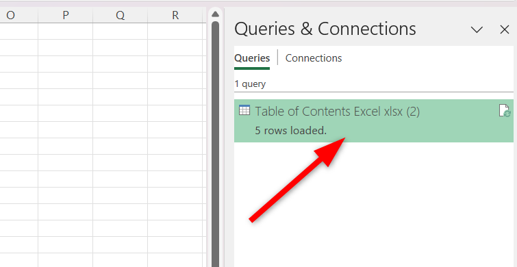
In the opened menu, click on “Refresh Preview” to update your Table of Contents.
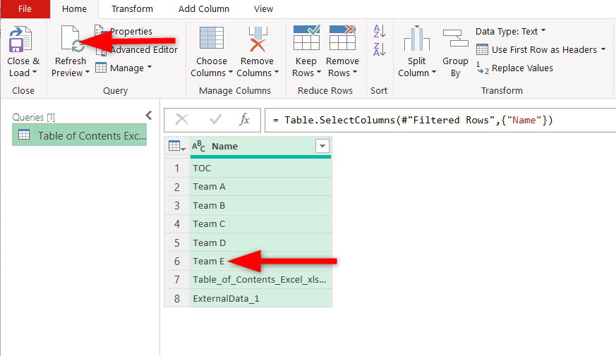
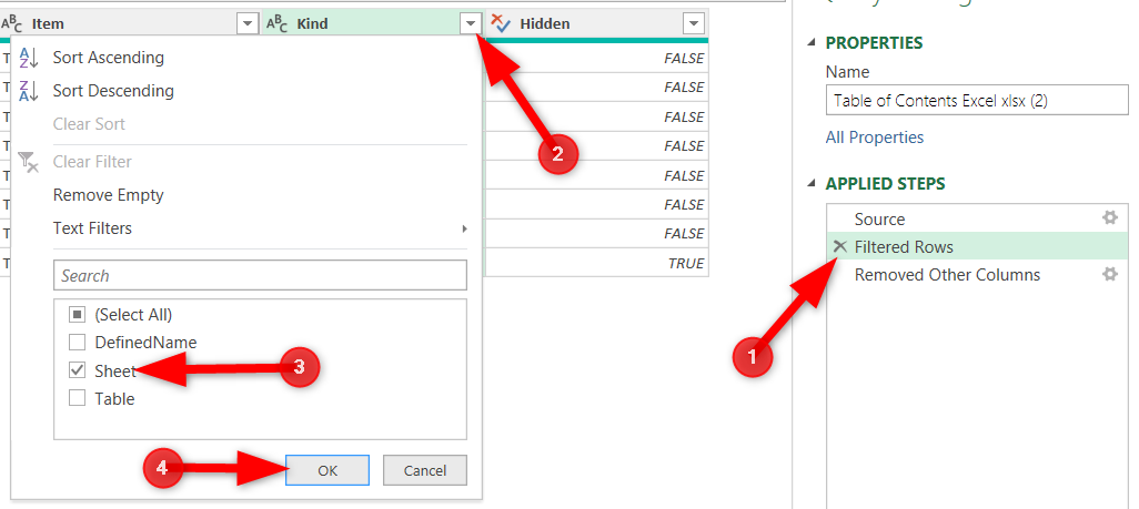
However, when you update it, any table or defined name recently added will also be included in the updated Table of Contents. To filter it, navigate to the “Filtered Rows” option, click on the “Kind” dropdown, and select only the “Sheet.”
That’s it! Power Query will automatically update the Table of Contents and include the newly added sheet.
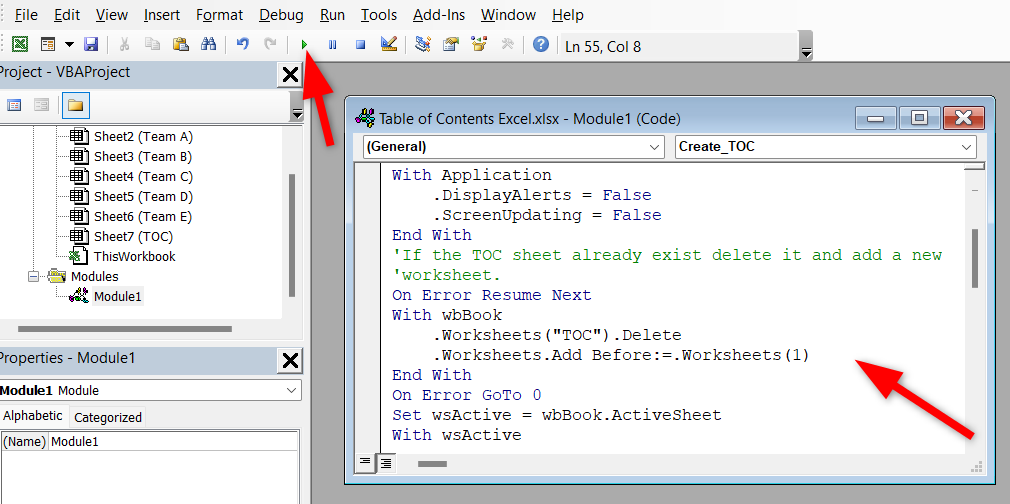
Use VBA Code Script
If your workbook is large, you can also use a VBA macro to automate the process by iterating through all sheets, creating a list entry for each, and inserting a hyperlink.
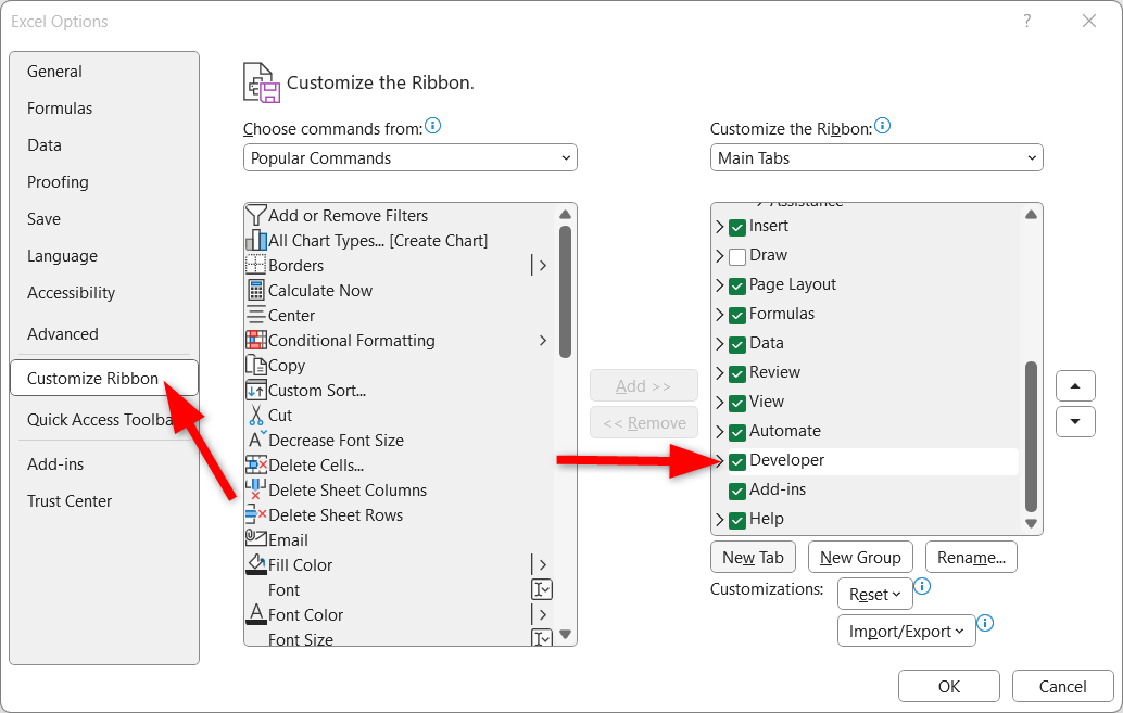
To add the VBA code, you need the Developer tab. If you’ve not accessed it before, it is not visible in the Ribbon. However, you can activate it by going to File > Options > Customize Ribbon and turning on the “Developer” option.
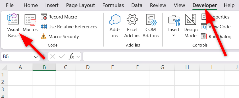
Next, head over to the Developer tab and select the “Visual Basic” option to open the VBA editor, or simply use the Alt+F11 shortcut.
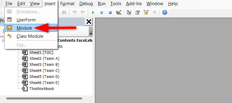
To insert a new module, click Insert > Module.
Finally, paste the VBA code provided by Dennis Wallentin into the editor window and click “Run” or press F5 to execute the code.
And that’s it! You’ve created a table of contents worksheet for your Excel workbook.
Create a Link Back to the TOC Sheet
If your workbook has many sheets, it can be helpful to add a hyperlink on each sheet that returns you to the master TOC page.
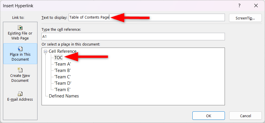
To begin, open the sheet where you want to add the return link and choose the cell where you need the link to display. Next, go to Insert > Link > Place in This Document. Select the master sheet and type “Table of Contents Page” as the display text.
You’ve now created a link that, when clicked, returns you to your main Table of Content page. You can easily copy this link and paste it on all other sheets.
Whether you’re dealing with a few sheets or a large workbook, these provided methods will help you create a table of contents efficiently.