Excel has so many tools that finding the right ones can often slow your workflow. Indeed, some of Excel’s most useful tools are also the most hidden, and it can sometimes take five or more clicks to perform a single action. This is why using the Quick Access Toolbar (QAT) is the way forward.
While the search bar at the top of the Excel window can help you find and perform an action, it’s sometimes difficult to know which keywords to use if you don’t remember the name of a function. Another option is to learn and use keyboard shortcuts, but since there are so many, they can take time to learn, and it can be difficult to recall which one to use. On the other hand, having buttons in the QAT means you can perform actions with just one click.
Which icons you add to your QAT will depend on what you use Excel for, but there are some that—in my opinion—are beneficial to everyone creating a spreadsheet.
As of July 2024, the QAT is only available in the Excel desktop app, and not Excel for the web.
Activate and Customize the Quick Access Toolbar
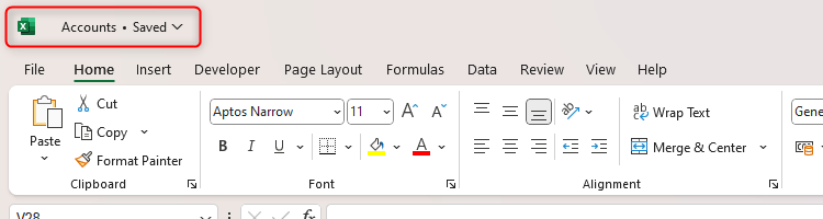
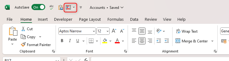
The QAT is in the top-left corner of your Excel window. If all you can see is the Excel logo and the name of your workbook, it means you don’t have the QAT enabled.
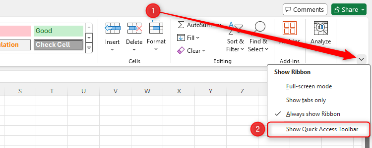
To rectify this, click the down arrow at the right-hand side of any of the open tabs, and click “Show Quick Access Toolbar.”
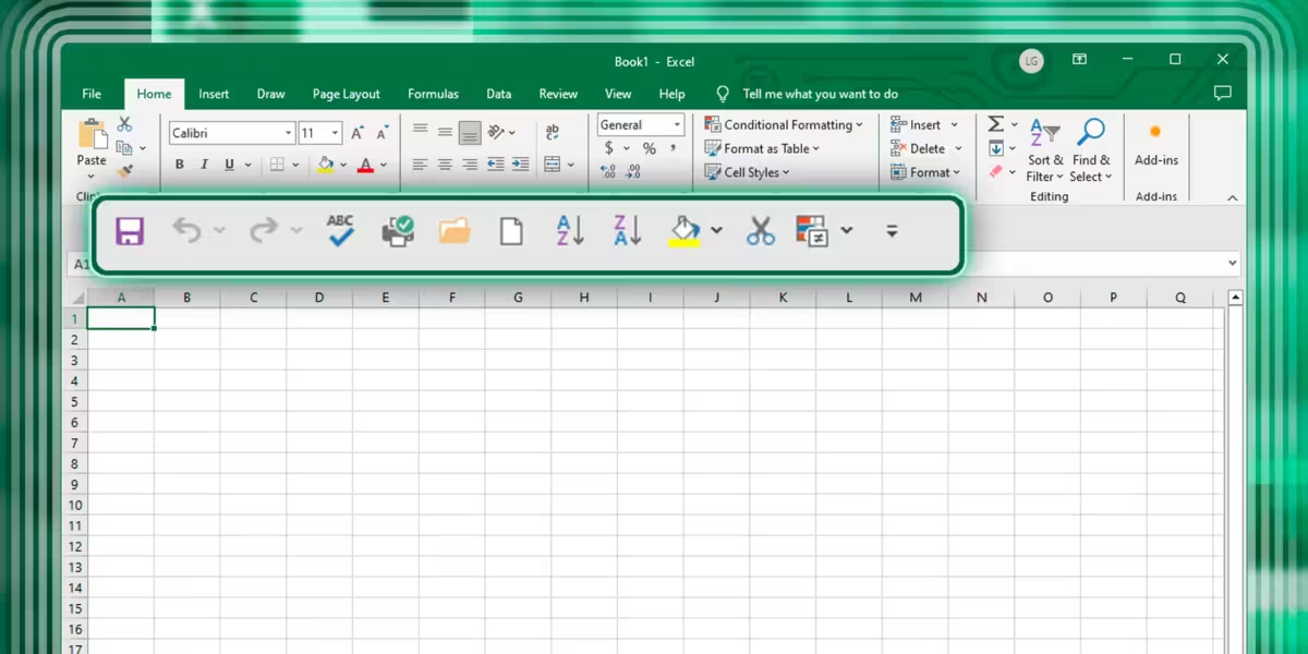
You will then see the QAT appear next to the Excel logo with some buttons, such as AutoSave and Save, as the default options.
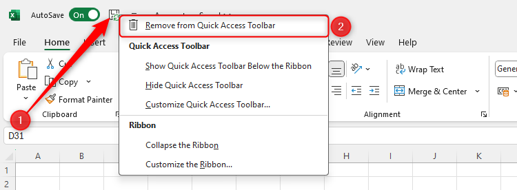
There are various ways to customize what you see here. To remove a button from your QAT, right-click the relevant icon and click “Remove From Quick Access Toolbar.”
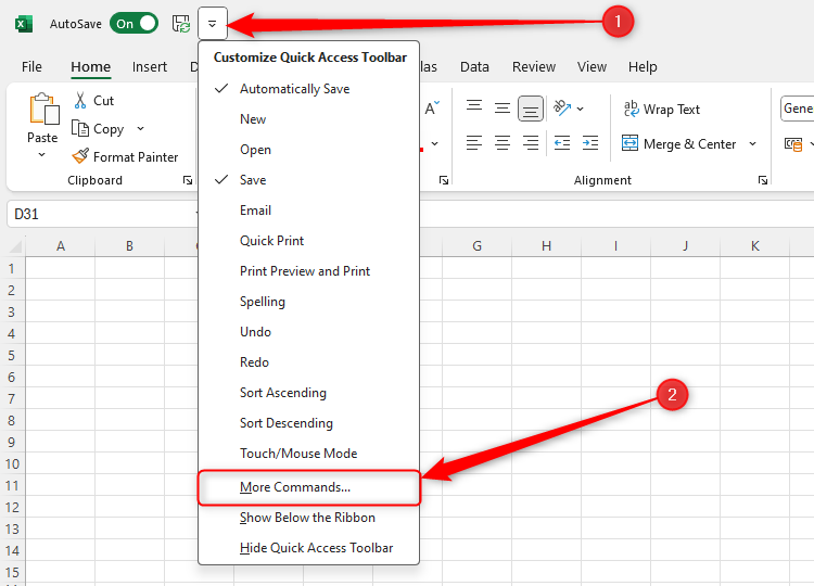
To add a button, click the “Customize Quick Access Toolbar” down arrow, and either choose one of the options available in that menu, or click “More Commands” to see the other actions you can add.

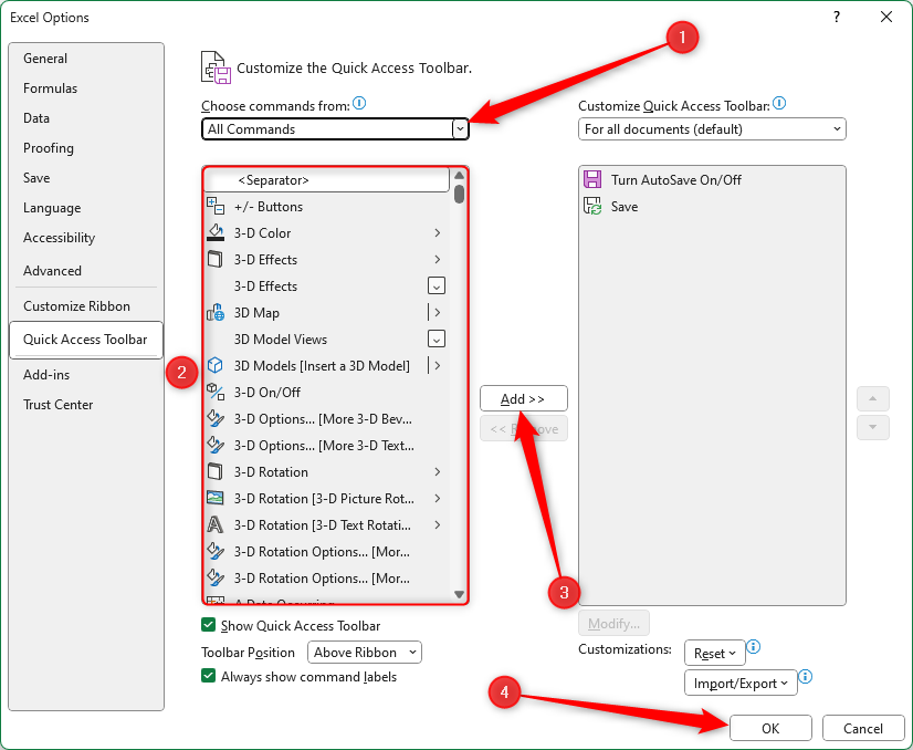
In the Excel Options window, click the “Choose Commands From” drop-down arrow to search for a tool by category or show all the available commands. Then, after finding and selecting a command you want to appear in your QAT, click “Add.” When you’re done, click “OK.”
You will then see the updated QAT based on your selections.
If you know where a command is located via the tabs on the ribbon, you can also right-click the command’s icon to add it to the QAT. Similarly, if you often use many commands from the same ribbon, you can add a whole ribbon’s icon to the QAT.
AutoSave
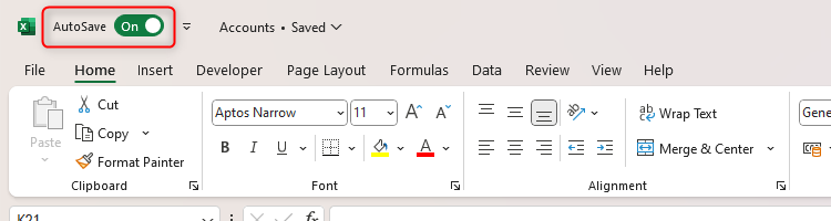
I find that having the AutoSave icon in the QAT is essential to ensure I don’t lose my work. If the AutoSave toggle is green, your work is saved and backed up to your OneDrive cloud.
However, if the AutoSave toggle is gray, your work isn’t currently syncing to the cloud, and you could lose your work if Excel crashes or your computer malfunctions.
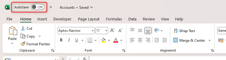
This could simply be because you’ve yet to save your work (Microsoft 365’s AutoSave only works once you’ve manually saved your work for the first time), so it’s a handy reminder to do this. If the AutoSave toggle is still set to Off, even after you have saved your work, it could mean one of three things:
- You have not signed in to your Microsoft account.
- You’re working on an outdated version of Excel (such as a 97-2003 Excel file), so you need to save the workbook in a more up-to-date format.
- There’s a OneDrive sync issue that you need to address outside of Excel by clicking the OneDrive icon in your Notification Center (the right-hand end of your Taskbar).
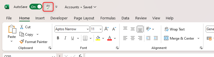
Spell Check
Unlike Microsoft Word, which instantly highlights spelling and grammar issues, Excel won’t tell you that you’ve made a typo because it is more interested in numbers and data. As a result, spelling errors can slip under the radar, which might have a detrimental impact on your spreadsheet’s functionality if, for example, you’re applying the IF function to the text containing the mistake. At the most basic level, if you’re sharing or printing your spreadsheet, you want it to be free of spelling issues.
So, adding the Spelling icon to the QAT serves as a crucial reminder to check your work for issues.
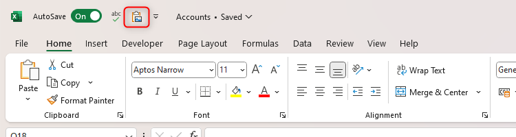
Paste Special
Ctrl+V is one of the most well-known keyboard shortcuts, but it’s less useful in Excel than in other programs. For example, you might want to copy and paste some data between sheets that are formatted differently, so you would want to paste the numbers without pasting the formatting. Similarly, you might only want to copy and paste the formatting, not the data. Going one step further, the Paste Special operation also lets you perform operations while pasting the data, such as turning all positive numbers into negative numbers.
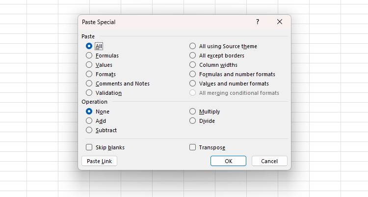
Because Paste Special lets you perform other actions while pasting information—such as removing formulas or borders—it’s an essential time-saving option in your QAT.
Conditional Formatting
Let’s be honest—if your Excel spreadsheet doesn’t have Conditional Formatting, it’s not really a proper Excel spreadsheet. Just as every Microsoft Word document should have styles, every Microsoft Excel worksheet should have Conditional Formatting, which is why the Conditional Formatting icon is a QAT non-negotiable.
Even if you don’t have the time (or the inclination!) to set up complex formatting rules based on cell values, using the preset Conditional Formatting options means you can analyze your data at a glance. For example, to apply each of the four types of Conditional Formatting to the data sets in the screenshot below, I simply had to select the array, click the Conditional Formatting icon in the QAT, and choose the format style.
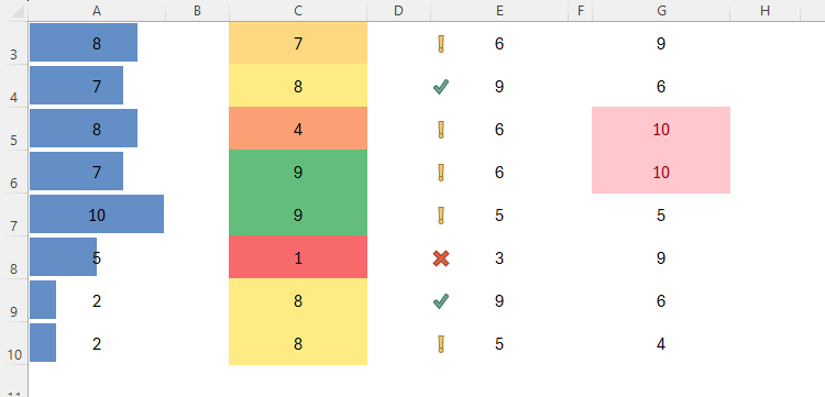
Having instant access to Conditional Formatting meant that the above actions took no more than five seconds, which is why you should also add this function to your QAT.
Freeze Panes
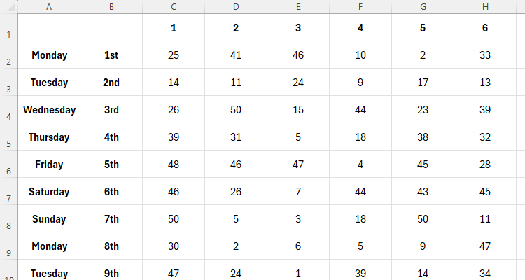
If you have a large spreadsheet with many rows and columns of data, it’s handy to freeze your heading rows and columns so that they remain in view when you scroll down or across. I always forget where the Freeze Panes option is—it feels like it should be in the Home tab (because it’s such a handy tool) or in the Data tab (because it helps you to read your data efficiently), but it’s actually in the View tab. So, having it in my QAT means I don’t have to go searching for it each time.
In this example, I want to freeze row 1 and columns A and B.
With cell C2 selected, I can click the Freeze Panes icon in the QAT and choose “Freeze Panes.” This option freezes all rows above and all columns to the left of the selected cell.
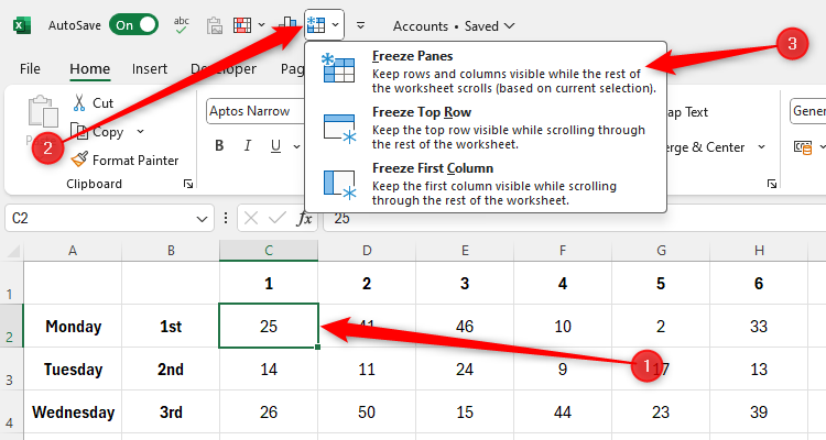
Notice, also, how you can instantly freeze just the first row or column using this handy QAT icon. Once you’ve frozen the relevant rows or columns, clicking the Freeze Panes icon in the QAT again will give you the option to unfreeze.
Personalized Macro Buttons
Microsoft 365’s macros let you perform very specific actions with one click. What’s more, Excel lets you add personalized macro buttons to your QAT, so it’s even easier to action that command.
Once you have recorded your macro, click the “Customize Quick Access Toolbar” down arrow, and choose “More Commands.”
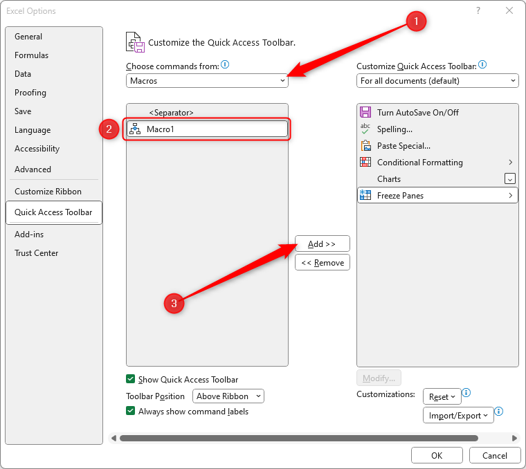
Then, in the Excel Options window, click the “Choose Commands From” drop-down arrow, and click “Macros.” Now, select the relevant macro, and click “Add.”
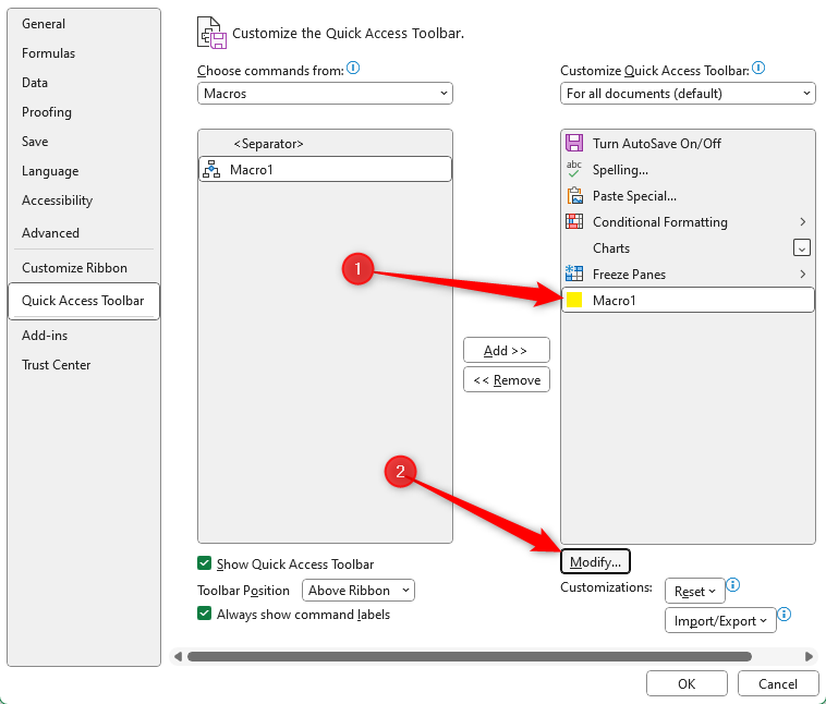
You can then choose a suitable icon for your macro by selecting the macro and clicking “Modify.” In the example below, the macro turns the selected cell yellow, so I have chosen a yellow icon.
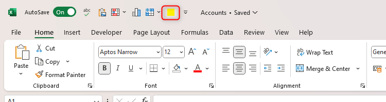
When you’re done, click “OK,” and you’ll see the new icon appear in your QAT.
You cannot modify QAT icons for standard commands—Excel only lets you change your personalized macro icons.
Reorder Icons in Your QAT
Once you have added all the relevant buttons to your QAT, consider reordering them so that using them is even easier. Personally, I order them by frequency of use, but you might choose to order them by type of command or to separate similar icons.
Click the down arrow next to your QAT, and click “More Commands” to open Excel Options.
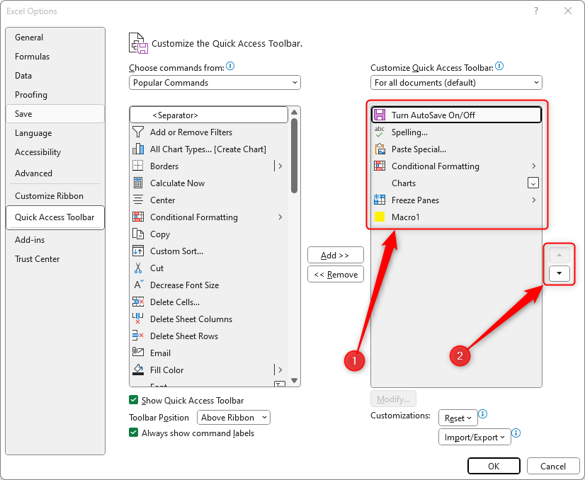
Then, select one of the icons already in your QAT, and use the arrows to choose your order. The icons at the top of the list will appear on the left of your QAT, and the icons at the bottom will appear on the right.
When you’re done, click “OK.”
By default, the QAT is right at the top of your Microsoft 365 app’s window. However, consider moving it to the bottom of the ribbon to make it even more accessible and speed up your work even further.